Wideband Tympanometry Research License

This guide is valid from Titan 3.5.

The Titan IMP440 WBT software comes with a possibility to export data to Matlab from the Wideband tympanometry tests. Here only the WB Absorbance and the 3D Tympanometry tests allows for data export. The following document describes how to setup the software for export and how to access the data in Matlab.

Start the Titan Suite and select the IMP tab in the right side of the screen.

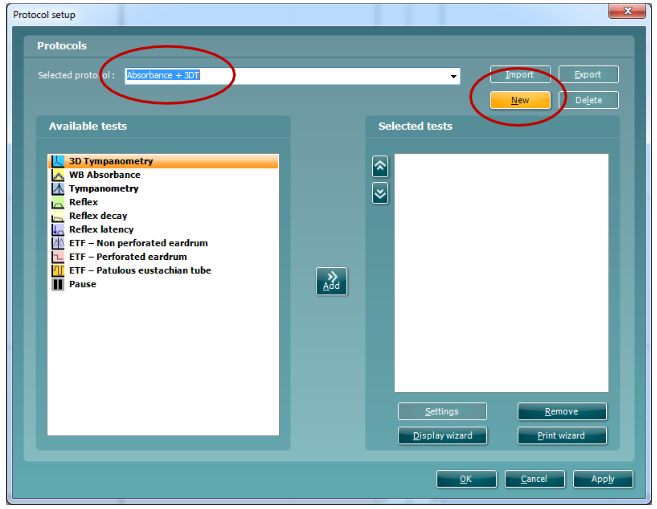
To setup a protocol go to Menu – Setup – Protocol setup.

Setup a new test – press New and type in the name of the test.

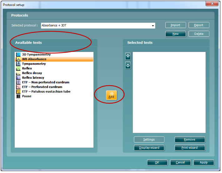
Add the test to the protocol pressing Add.

Note that while obtaining data with multiple protocols e.g. WBT, reflexes and ETF, it is only the wideband tympanometry or absorbance data that gets exported in the research file.

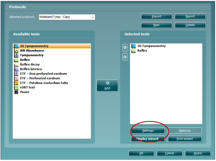
Press Settings to change settings.

In the settings, ensure the Save measurement to research file box is ticked off to save a research file in the specified folder. The folder can be changed as desired.

The rest of the settings are as described in the Titan manual.

Press Ok to save the settings when finished.

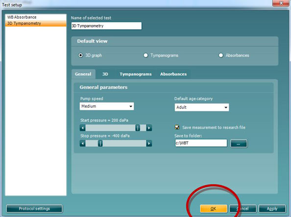
Press Ok again to save the completed test protocol.

Start the test by pressing the Start button

When the test protocol is done, two files are saved in the specified folder by default e.g. C:\WBT.

The WB Absorbance file is labeled “File_WBA_YYYY_MM_DD_HH_MM_SS.m”, with a time-stamp of the measurement time. The 3D Tympanometry file is labeled “File_WB3DT_YYYY_MM_DD_HH_MM_SS.m”, with a time-stamp of the measurement time.

NB: The time-stamp is NOT equal to the time-stamp in the session list when saving the session!

To export data to Matlab, start up Matlab, and set the folder to the specified folder (default C:\WBT):

Type the file name in the command window of the specified test file (without the .m-file extension) and press enter:

All data in the .m-file is loaded into a struct with the same name as the file (except for the prefix “File_”). Type in the struct name to view its members:

The frequency dependent energy Absorbance data is located in the member “ABS”, and the frequency data in “FREQ”. The frequency dependent complex admittance is located in the “ADMITTANCE_MAG” and “ADMITTANCE_ANGLE”. Data are in 1/24th octave frequency resolution with some octave frequencies absent in the low frequencies. The frequency range is 226 Hz to 8000 Hz.

For the 3D Tympanometry measurement, type the file name in the command window of the specified test file (without the .m-file extension) and press enter. All data in the .m-file is loaded into a struct with the same name as the file (except for the prefix “File_”). Type in the struct name to view its members:

*The reflectance allows for calculation of the absorbance. However, if going from the reflectance to the absorbance the values of absorbance provided and the one calculated of the reflectance will deviate. This is caused by a filtering for the absorbance values provided.

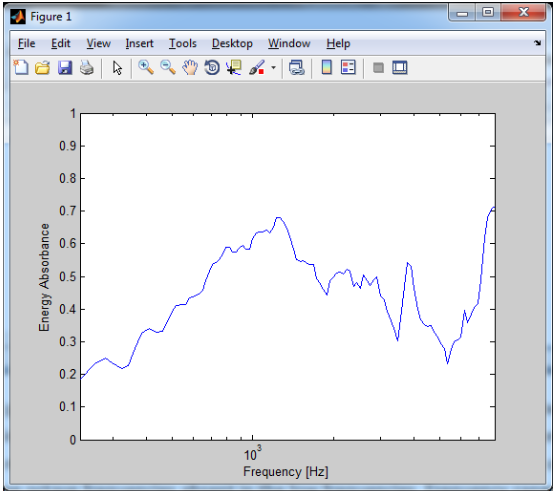
To view Absorbance data, type the following in the Matlab Command Window:

semilogx( WBA_2013_05_07__15_38_13.FREQ, WBA_2013_05_07__15_38_13.ABS ) axis([226 8000 0 1])
xlabel('Frequency [Hz]')
ylabel('Energy Absorbance')

The following is plotted:

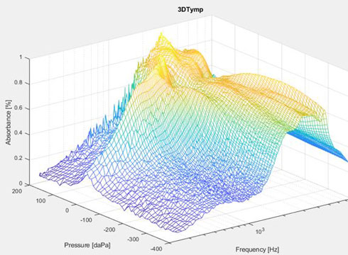
To view 3D Tympanometry data, type the following in the Matlab Command Window:

mesh(log10(WB3DT_2013_05_07__15_38_26.FREQ), ... -WB3DT_2013_05_07__15_38_26.PRESSURE, WB3DT_2013_05_07__15_38_26.ABSORBANCE )

set(gca,'XTick',log10([250, 500,1000,2000,4000,8000])) set(gca,'XTickLabel',{'250','500','1k','2k','4k','8k'}) set(gca,'YTick',[-200,-100,0,100,200,300,400]) set(gca,'YTickLabel',{'200','100','0','-100','-200','-300','-400'}) axis([log10(250) log10(8000) -200 400 0 1]) xlabel('Frequency [Hz]')

ylabel('Pressure [daPa]') ylabel('Energy Absorbance')

The following is plotted:

To plot the data based on the reflectance data, the following script can be used.

1) To see the 3Dtympanometry graph by the use of the reflectance data, the following script can be used.

%Run the file you want to analyse File_WB3DT_....... in the same folder as %this script.

TitanTestResult = WB3DT_2019_09_18__14_26_22;%Rename this line WB3DT.... to one above TitanTestResult.REFLECTANCE = (TitanTestResult.REFLECTANCE');

absorbance = 1 - TitanTestResult.REFLECTANCE .* conj(TitanTestResult.REFLECTANCE); absorbance(absorbance<0)=0;

figure;mesh(TitanTestResult.REFLECTANCE_FREQUENCIES, TitanTestResult.PRESSURE, absorbance');

title('3dt example');xlabel('frequency [Hz]');ylabel('Pressure [daPa]');zlabel('Absorbance [%]'); set(gca,'XScale','log');
xlim([200 9000]);

2) To plot the data based on the absorbance, the following script can be used.

%Run the file you want to analyse File_WB3DT_....... in the same folder as %this script.

TitanTestResult = WB3DT_2019_09_18__14_26_22;%Rename this line WB3DT.... to one above

TitanTestResult.REFLECTANCE = (TitanTestResult.REFLECTANCE');

%find Absorbance

absorbance = 1 - TitanTestResult.REFLECTANCE .* conj(TitanTestResult.REFLECTANCE); absorbance(absorbance<0)=0;

figure;mesh(TitanTestResult.REFLECTANCE_FREQUENCIES, TitanTestResult.PRESSURE, absorbance');

title('3DTymp');xlabel('Frequency [Hz]');ylabel('Pressure [daPa]');zlabel('Absorbance [%]'); set(gca,'XScale','log');
xlim([200 8000]);

DesiredFreq = 2000; %Set the desired frquency
%find nearest fequency index
[ ~, indexOfxxxkHz ] = min( abs( TitanTestResult.REFLECTANCE_FREQUENCIES-DesiredFreq ) )
%find Admittance
admittance = (((1+0i)- TitanTestResult.REFLECTANCE(indexOfxxxkHz,:))./(((1+0i)+TitanTestResult.REFLECTANCE(indexOfxxxk Hz,:)).* TitanTestResult.Z0_CALIBRATION(indexOfxxxkHz))).';
y = abs(admittance);

figure;plot(TitanTestResult.PRESSURE, y*1000)
title('2 kHz Tympanogram');xlabel('Pressure [daPa]');ylabel('[mmho]'); grid on

3) To plot the data of a tympanogram, the following script can be used.

%Run the file you want to analyse File_WBA_....... in the same folder as %this script.

TitanTestResult = WBA_2019_09_18__14_26_28;%rename this line WBA.... to one above TitanTestResult.REFLECTANCE = (TitanTestResult.REFLECTANCE');

absorbance = 1 - TitanTestResult.REFLECTANCE .* conj(TitanTestResult.REFLECTANCE); absorbance(absorbance<0)=0;

figure;semilogx(TitanTestResult.REFLECTANCE_FREQUENCIES,mean(absorbance,2)); grid on; xlim([200 9000]); ylim([0 1])
title('Absorbance example');xlabel('frequency [Hz]');ylabel('Absorbance [%]');