What is Auditory Brainstem Response (ABR) Testing?

This video provides an overview of the basic theory of threshold auditory brainstem response (ABR) testing, with a focus on testing the newborn baby population.

If you prefer reading, please find the full transcript below.

What is the auditory brainstem response (ABR)?

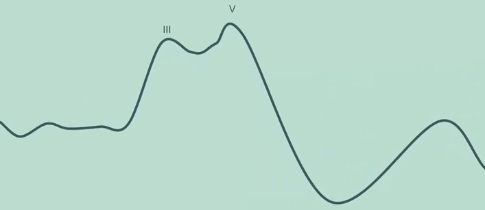
The auditory brainstem response (ABR) is an action potential generated by the brainstem in response to the presentation of an auditory stimulus. The auditory brainstem response is made up of a series of seven peaks and troughs which are generated by neural firing at different – but sometimes overlapping – stages of the pathway (Figure 1).

ABR waves

Waves VI and VII are of little clinical utility, leaving waves I-V as those focused on in clinical practice. Wave V is the primary focus of threshold ABR testing being the largest peak and thus easiest to detect.

ABR amplitude

The ABR is unaffected by sleep so can theoretically be recorded when the patient is awake or asleep. However, it is a relatively small evoked potential response. Certainly in comparison to responses generated by the cortical region, which show much larger amplitudes.

Because of the small nature of the ABR amplitude, it can be easily lost within any other noise that may be recorded by the system. This means that testing with an asleep or very settled patient is recommended to ensure good quality recordings can be obtained.

ABR morphology

The shape of the ABR is known as the morphology. Figure 1 above is a textbook example but more often than not in clinical practice, the ABR response can look very different to this, and you can expect to see significant variability between patients.

Sometimes only waves III and V can be clearly distinguished within the waveform (Figure 2).

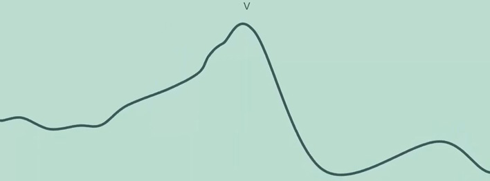
Frequently however, only wave V can be identified (Figure 3).

ABR results interpretation

Depending on:

• Stimulus type
• Frequency
• Intensity level
• Degree and type of hearing loss

Many different ABR morphologies can be recorded, and this can make waveform interpretation challenging for new or inexperienced testers. The key to determining whether an ABR response is present – and thus whether the patient can hear the sound being presented to their ear – is by identifying wave V.

How to identify wave V

There are some fundamental principles that can help in this process.

1. Morphology

Firstly, the morphology of the ABR matters. It should look and feel like an ABR on the screen, particularly the characteristic wave V peak followed by the trough dropping off shortly afterwards. Noisy waveforms can make this harder to see, so good recording conditions are really important to help with waveform interpretation.

2. Latency

The latency or timing of wave V should be roughly around seven to nine milliseconds. There is normative data available in the literature and built in to some evoked potential testing devices. But this isn't always available for every stimulus type and age group.

It is also common to see latency values out of the ordinary in certain types of hearing losses. A conductive hearing loss for instance is likely to present with much longer latencies than normal hearing. It is important to be able to differentiate between a wave V that may not match the normative data and a spike of noise within the waveform.

3. Amplitude

The amplitude of the waveform is taken from the peak of wave V to the trough that immediately follows wave V. The trough is typically present at a latency of 10 milliseconds, but this can be variable. Typically, ABR amplitudes are between 0.1 and 1 microvolt. In some countries, an amplitude of 0.04 microvolts is used as the minimum acceptance criteria for determining if wave V is present.

4. Latency shift

One of the most valuable tools for determining whether a response is present is to look at neighboring intensity levels. An expected pattern of results is to see a latency shift with varying intensity.

Wave V should appear at shorter latencies for louder intensities and at longer latencies for quieter intensities. An amplitude decrease is also expected for quieter intensities and by the same token an increase in amplitude should be seen for louder intensities.

In Figure 4, we have three different intensity levels for the same stimulus. In this instance, the waveforms recorded are good quality with minimal noise and no baseline drift making it easy to identify wave V.

At the level of 60, we can see wave V is present at just before 8 milliseconds. By decreasing the intensity level to 40, we can see that the latency of wave V has shifted to the right. In other words, it is a longer latency. Here, wave V presents at about 8.5 milliseconds (Figure 5).

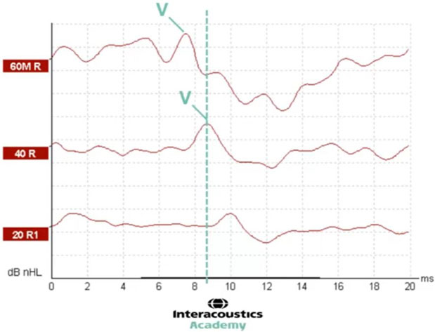
With a further decrease in intensity, we can see that the latency of wave V has shifted even further to the right, presenting at 10 milliseconds. This demonstrates the expected latency shift as a function of decreasing intensity (Figure 6).

5. Amplitude change

We can also see the amplitude change in this example. At the level of 60, we can highlight wave V and the trough and measure the amplitude as the difference between them (Figure 7).

By dropping to a quieter intensity of 40 dB nHL, it is possible to see that the amplitude of this waveform is smaller than that recorded at 60 (Figure 8).

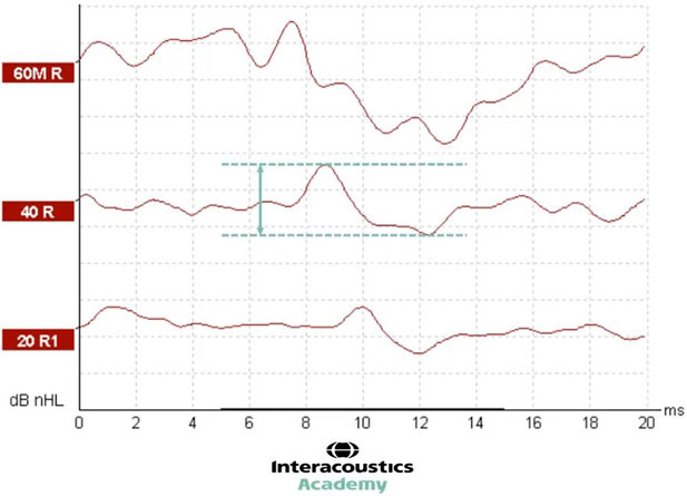
And with a further decrease to 20 dB nHL, the waveform amplitude decreases further yet again (Figure 9).

This demonstrates the expected decrease in amplitude when decreasing the intensity level.

By looking for these changes in amplitude and latency, this can help to provide confirmation that wave V has been identified correctly and that the ABR response is behaving as expected. If a set of waveforms do not follow this pattern of results, then further investigation on why is warranted:

• Has there been a technical issue?
• Has wave V been marked incorrectly?
• Do the waveforms contain too much noise?
• Could there be a more complex or unusual type of hearing loss present?

Other tools

There are two objective tools available to assist in determining whether a response is present.

1. FMP

FMP is a statistical calculation provided by the Eclipse software which looks at the likelihood of an ABR being present for newborn babies. A minimum value of 7 is recommended and at least 800 sweeps must be recorded before the FMP value is read.

2. Residual noise

The residual noise within a waveform is also calculated by the Eclipse software. This provides an indication of the quality of the waveform. The lower the residual noise, the better the quality. This can help to guide whether further testing is required to improve the quality of the waveform or whether a sufficiently good quality waveform has been recorded and testing can thus stop. This is particularly valuable when there appears to be no ABR present.

To determine that there is no response, the waveform must be sufficiently lacking in noise to minimize the possibility of a small response being hidden within a noisy waveform. Once the residual noise has reached a suitably low level, the clinician can have confidence that there is minimal noise within which an ABR could be hidden. It is advisable to refer to local guidelines for recommended residual noise stop criteria. However, many clinics use between 15 and 25 nanovolts for newborn babies.